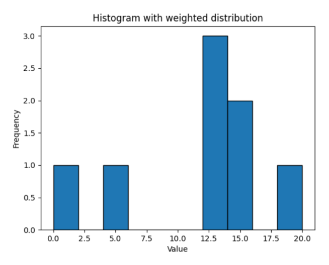
The numpy.histogram() method computes the histogram of a dataset.
Example
import numpy as np

array1 = np.array([0, 12, 14, 17, 12, 4, 3, 3, 13, 12, 9, 17, 14, 11, 5, 20])

# compute histogram of array1
graph= np.histogram(array1)

print(graph)

# Output: (array([1, 2, 2, 0, 1, 1, 4, 2, 2, 1]), array([ 0.,  2.,  4.,  6.,  8., 10., 12., 14., 16., 18., 20.]))
histogram() Syntax
The syntax of the numpy.histogram() method is:
numpy.histogram(array, bins = 10, range = None, density = None, weights = None)
histogram() Arguments
The numpy.histogram() method takes the following arguments:
array- input array (array_like)bins(optional) - number of equal width bins in a range (intorsequence of scalarsorstr)range(optional) - the lower and upper range of the bins ((float, float))density(optional) - specifies whether the returned histogram values should be normalized to form a probability density (bool)weights(optional) - the array of weights having the same shape asarray(array_like)
histogram() Return Value
The numpy.histogram() method returns the values of histogram.
Histogram
A histogram graphically represents the frequency distribution of numerical data.
Histograms are similar to bar graphs. But unlike bar graphs (that represent absolute values), each bar in a histogram represents a certain range.
In NumPy, we use the histogram() function to calculate the frequency distribution of data, which we can then show in the form of a graph.
Example 1: NumPy Histogram
If we pass a sequence as bins, the sequence in ascending order acts as the bin edges for the distribution.
import numpy as np

# create an array of data
data = np.array([5, 10, 15, 18, 20])

# create bin to set the interval
bin = [0,10,20,30]

# create histogram
graph = np.histogram(data, bin)

print(graph)
Output
(array([1, 3, 1]), array([ 0, 10, 20, 30]))
The histogram() method returns a tuple containing two arrays:
- The first array contains the frequency counts of the data within each bin.
- The second array contains the bin edges.
In the example above,
- The first bin has a range of [0, 10) and 1 item (5).
- The second bin has a range of [10, 20) and 3 items (10, 15, 18).
- The final bin has a range of [20, 30] and 1 item (20).
Example 2: NumPy Histogram With range
In our previous examples, the histogram ranged from the array's minimum value to the maximum value.
However, we can manually specify the range of the histogram using the range argument.
import numpy as np
array1 = np.array([0, 12, 14, 17, 12, 4, 3, 3, 13, 12, 9, 17, 14, 11, 5, 20])

# compute histogram from 0 to 30
graph= np.histogram(array1, range = (0, 30))

print(graph)
Output
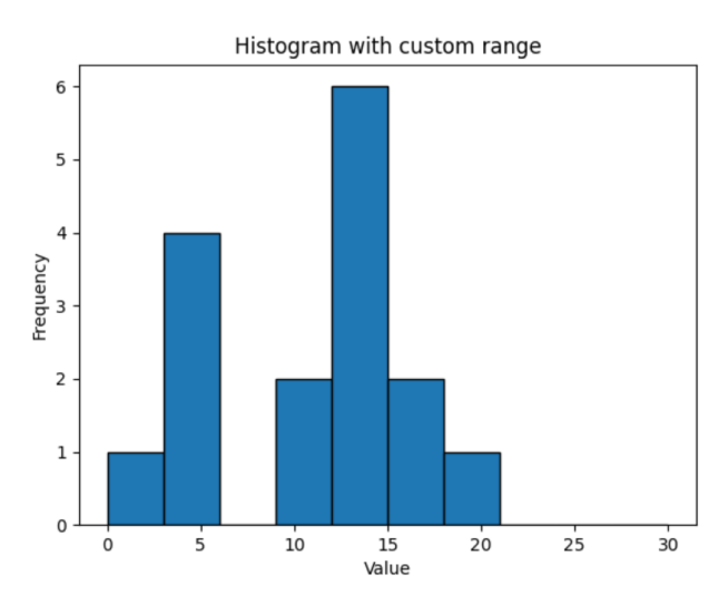
(array([1, 4, 0, 2, 6, 2, 1, 0, 0, 0]), array([ 0., 3., 6., 9., 12., 15., 18., 21., 24., 27., 30.]))
Note: Both start and stop values in range are included in bins.
Example 3: NumPy Histogram With density
We can normalize the returned histogram values to form a probability density if we set the density argument to True (density = True).
import numpy as np

array1 = np.array([0, 12, 14, 17, 12, 4, 3, 3, 13, 12, 9, 17, 14, 11, 5, 20])

# compute histogram
graph= np.histogram(array1)

print('Unnormalized Distribution:\n', graph)

# compute histogram with density = True
graph= np.histogram(array1, density = True)

print('Normalized Distribution:\n', graph)
Output
Unnormalized Distribution:
(array([1, 2, 2, 0, 1, 1, 4, 2, 2, 1]), array([ 0.,  2.,  4.,  6.,  8., 10., 12., 14., 16., 18., 20.]))
Normalized Distribution:
(array([0.03125, 0.0625 , 0.0625 , 0.     , 0.03125, 0.03125, 0.125  ,
       0.0625 , 0.0625 , 0.03125]), array([ 0.,  2.,  4.,  6.,  8., 10., 12., 14., 16., 18., 20.]))
Example 4: NumPy Histogram With weights
All elements of the array ideally have equal weights in the histogram. However, we can assign weights to each element using the weights argument.
import numpy as np

array1 = np.array([0, 12, 14, 17, 12, 4, 3, 3, 13, 12, 9, 17, 14, 11, 5, 20])

# compute histogram
graph= np.histogram(array1)

print('Equal Weights:\n', graph)

# compute histogram with even weights = 1 and odd weights = 0
weights = np.where(array1 % 2 == 0, 1, 0)
graph= np.histogram(array1, weights = weights)

print('Weighted Distribution:\n', graph)
Output
Equal Weights:
(array([1, 2, 2, 0, 1, 1, 4, 2, 2, 1]), array([ 0.,  2.,  4.,  6.,  8., 10., 12., 14., 16., 18., 20.]))
Weighted Distribution:
(array([1, 0, 1, 0, 0, 0, 3, 2, 0, 1]), array([ 0.,  2.,  4.,  6.,  8., 10., 12., 14., 16., 18., 20.]))
Example 5: Visualization of Histogram
We can use matplotlib to visualize the histogram data.
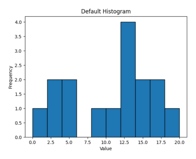
Default Histogram
import numpy as np
import matplotlib.pyplot as plt

# define array
array1 = np.array([0, 12, 14, 17, 12, 4, 3, 3, 13, 12, 9, 17, 14, 11, 5, 20])

# compute histogram
counts, bin_edges = np.histogram(array1)

# plot histogram using counts and bin_edges
plt.bar(bin_edges[:-1], counts, width=np.diff(bin_edges), align='edge', edgecolor='black')
plt.title('Default Histogram')
plt.xlabel('Value')
plt.ylabel('Frequency')

plt.show()
Output
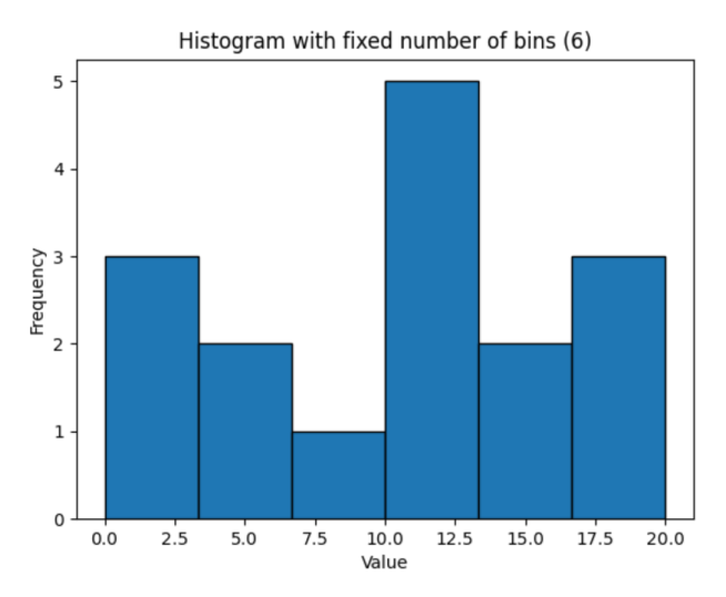
Histogram With Fixed Number of Bins
import numpy as np
import matplotlib.pyplot as plt

# define array
array1 = np.array([0, 12, 14, 17, 12, 4, 3, 3, 13, 12, 9, 17, 14, 11, 5, 20])

# compute histogram by specifying the number of bins(6)
counts, bin_edges = np.histogram(array1, bins=6)

# plot histogram using counts and bin_edges
plt.bar(bin_edges[:-1], counts, width=np.diff(bin_edges), align='edge', edgecolor='black')
plt.title('Histogram with fixed number of bins (6)')
plt.xlabel('Value')
plt.ylabel('Frequency')

plt.show()
Output
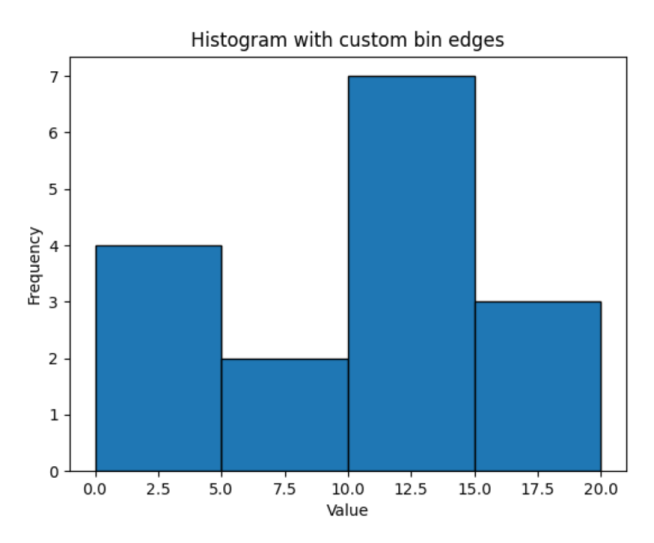
Histogram With Custom Bin Edges
import numpy as np
import matplotlib.pyplot as plt

# define array
array1 = np.array([0, 12, 14, 17, 12, 4, 3, 3, 13, 12, 9, 17, 14, 11, 5, 20])

# create custom bin edges
bins = [0, 5, 10, 15, 20]
counts, bin_edges = np.histogram(array1, bins=bins)

# plot histogram using custom bin edges
plt.bar(bin_edges[:-1], counts, width=np.diff(bin_edges), align='edge', edgecolor='black')
plt.title('Histogram with custom bin edges')
plt.xlabel('Value')
plt.ylabel('Frequency')

plt.show()
Output
Histogram With Custom Range
import numpy as np
import matplotlib.pyplot as plt

# define array
array1 = np.array([0, 12, 14, 17, 12, 4, 3, 3, 13, 12, 9, 17, 14, 11, 5, 20])

# compute histogram with fixed range (0 to 30)
counts, bin_edges = np.histogram(array1, range=(0, 30))

plt.bar(bin_edges[:-1], counts, width=np.diff(bin_edges), align='edge', edgecolor='black')
plt.title('Histogram with custom range')
plt.xlabel('Value')
plt.ylabel('Frequency')

plt.show()
Output
Histogram With Normalized Distribution
import numpy as np
import matplotlib.pyplot as plt

# define array
array1 = np.array([0, 12, 14, 17, 12, 4, 3, 3, 13, 12, 9, 17, 14, 11, 5, 20])

# compute histogram with density
counts, bin_edges = np.histogram(array1, density=True)

plt.bar(bin_edges[:-1], counts, width=np.diff(bin_edges), align='edge', edgecolor='black')
plt.title('Histogram with normalized distribution')
plt.xlabel('Value')
plt.ylabel('Frequency')

plt.show()
Output

Histogram With Weighted Distribution
import numpy as np
import matplotlib.pyplot as plt

# define array
array1 = np.array([0, 12, 14, 17, 12, 4, 3, 3, 13, 12, 9, 17, 14, 11, 5, 20])

# compute histogram with even weights = 1 and odd weights = 0
weights = np.where(array1 % 2 == 0, 1, 0)
counts, bin_edges = np.histogram(array1, weights=weights)

plt.bar(bin_edges[:-1], counts, width=np.diff(bin_edges), align='edge', edgecolor='black')
plt.title('Histogram with weighted distribution')
plt.xlabel('Value')
plt.ylabel('Frequency')

plt.show()
Output
